45 change order of data labels in excel chart
› documents › excelHow to change/edit Pivot Chart's data source/axis/legends in ... Actually, it's very easy to change or edit Pivot Chart's axis and legends within the Filed List in Excel. And you can do as follows: Step 1: Select the Pivot Chart that you want to change its axis and legends, and then show Filed List pane with clicking the Filed List button on the Analyze tab. support.microsoft.com › en-us › officeAdd or remove data labels in a chart - support.microsoft.com Click the data series or chart. To label one data point, after clicking the series, click that data point. In the upper right corner, next to the chart, click Add Chart Element > Data Labels. To change the location, click the arrow, and choose an option. If you want to show your data label inside a text bubble shape, click Data Callout.
Data Labels in Excel Pivot Chart (Detailed Analysis) Clicking on any Data labels one time will select all of the Data Labels simultaneously. Then right-click on the Data Table and from the context menu, click on the Format Data Labels. Then in the Format Data Labels, go to the Size and Properties. From there, click on the Text Directions. And from the drop-down menu, click on the Rotate all text 270.

Change order of data labels in excel chart
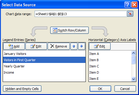
Change the labels in an Excel data series | TechRepublic Click the Chart Wizard button in the Standard toolbar. Click Next. Click the Series tab. Click the Window Shade button in the Category (X) Axis. Labels box. Select B3:D3 to select the labels in ... How to reverse order of items in an Excel chart legend? - ExtendOffice Right click the chart, and click Select Data in the right-clicking menu. See screenshot: 2. In the Select Data Source dialog box, please go to the Legend Entries (Series) section, select the first legend ( Jan in my case), and click the Move Down button to move it to the bottom. 3. Repeat the above step to move the originally second legend to ... Excel charts: add title, customize chart axis, legend and data labels Click anywhere within your Excel chart, then click the Chart Elements button and check the Axis Titles box. If you want to display the title only for one axis, either horizontal or vertical, click the arrow next to Axis Titles and clear one of the boxes: Click the axis title box on the chart, and type the text.
Change order of data labels in excel chart. Edit titles or data labels in a chart - support.microsoft.com The first click selects the data labels for the whole data series, and the second click selects the individual data label. Right-click the data label, and then click Format Data Label or Format Data Labels. Click Label Options if it's not selected, and then select the Reset Label Text check box. Top of Page How to Change Excel Chart Data Labels to Custom Values? - Chandoo.org Now, click on any data label. This will select "all" data labels. Now click once again. At this point excel will select only one data label. Go to Formula bar, press = and point to the cell where the data label for that chart data point is defined. Repeat the process for all other data labels, one after another. See the screencast. Points to note: Bar chart Data Labels in reverse order - Microsoft Tech Community The order in which the text appears in these cells is the order that the labels will be displayed. The cells from which the label values are taken are totally independent of the axis order. The first data item gets the first label. If you want to reverse the data order in the chart, you will need to build a corresponding list of labels. support.microsoft.com › en-us › officeChange the format of data labels in a chart To get there, after adding your data labels, select the data label to format, and then click Chart Elements > Data Labels > More Options. To go to the appropriate area, click one of the four icons ( Fill & Line , Effects , Size & Properties ( Layout & Properties in Outlook or Word), or Label Options ) shown here.
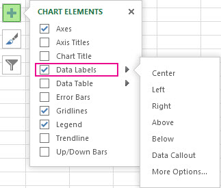
How to add or move data labels in Excel chart? - ExtendOffice In Excel 2013 or 2016. 1. Click the chart to show the Chart Elements button . 2. Then click the Chart Elements, and check Data Labels, then you can click the arrow to choose an option about the data labels in the sub menu. See screenshot: In Excel 2010 or 2007. 1. click on the chart to show the Layout tab in the Chart Tools group. See ... Change the plotting order of categories, values, or data series Click the chart for which you want to change the plotting order of data series. This displays the Chart Tools. Under Chart Tools, on the Design tab, in the Data group, click Select Data. In the Select Data Source dialog box, in the Legend Entries (Series) box, click the data series that you want to change the order of. › charts › pareto-templateHow to Create a Pareto Chart in Excel – Automate Excel To reposition the labels, right-click on the data labels for Series “Cumulative %” and choose “Format Data Labels.” In the Format Data Labels task pane, change the position of the labels by doing the following: Go to the Label Options tab. Under “Label Position,” choose “Above.” You can also change the color and size of the ... Arranging Trendline Labels in Excel Chart Legend - It won't follow ... Arranging Trendline Labels in Excel Chart Legend - It won't follow the Select Data order. I've got a chart in Excel on Windows that will not change the order of the entries in the legend. I've got scatterplots with trendlines and they're labeled "2017" on up to "2021" but for some reason 2019 will not go in the right order.
Change the Order of Data Series of a Chart in Excel - Excel Unlocked We can change this order. Right click on this chart and click on the Select Data option. After that select 2019 from the data series and click on the down arrow. This will move the data series 2019 below 2020. Click OK. As a result, you would see a change of order in your column chart as follows. This brings us to the end of the blog. Legend label order and chart data series order do not correspond The entries in the chart legend are different than the series order in the 'Legend Entries (Series)' column of the 'Select Data Source' dialog. Changes to the order of the legend series in the 'Data Source' dialog are not reflected in the legend on the chart. We have even deleted the legend and selected a new default legend, without any effect. Changing the order of items in a chart - PowerPoint Tips Blog Follow these steps: With the chart selected, click the Chart Tools Design tab. Choose Select Data in the Data section. The Select Data Source dialog box opens. You can only change the values on the left side of the dialog box, so you might have to click the Switch Row/Column button. How to change the order of data layer on chart Jan 26, 2007. #5. Thanks John, I am using a secondary axis for one of the series, so there isn't even two series listed to be able to change order. i've tried makeing the secondary primary, so then i can see the two in the orderlist, but when I swap first for second, it stil doesn't change the stacking order.
How to Make a Pie Chart in Excel – Contextures Blog
How to add data labels from different column in an Excel chart? Right click the data series in the chart, and select Add Data Labels > Add Data Labels from the context menu to add data labels. 2. Click any data label to select all data labels, and then click the specified data label to select it only in the chart. 3.

Add or remove data labels in a chart
How to change the order of your chart legend - Excel Tips & Tricks ... Under the Data section, click Select Data. Step 2: In the Select Data Source pop up, under the Legend Entries section, select the item to be reallocated and, using the up or down arrow on the top right, reposition the items in the desired order.
Change Data Series Order : Chart Data « Chart « Microsoft ...
How to create Custom Data Labels in Excel Charts - Efficiency 365 Create the chart as usual. Add default data labels. Click on each unwanted label (using slow double click) and delete it. Select each item where you want the custom label one at a time. Press F2 to move focus to the Formula editing box. Type the equal to sign. Now click on the cell which contains the appropriate label.

Highlight a Specific Data Label in an Excel Chart - Peltier Tech
Change order of data labels in chart - Microsoft Community Yes No TA tartan10 Replied on March 4, 2013 In reply to Ty_hell_heaven's post on March 4, 2013 The data were added in the order shown in the list before realizing that the labels could not be moved around. The order of the labels on the right should be, downward, 10, 8, 6, 4, and 2. Report abuse Was this reply helpful? Yes No TA tartan10

Change color of data label placed, using the 'best fit ...
Is there a way to change the order of Data Labels? Answer Rena Yu MSFT Microsoft Agent | Moderator Replied on April 4, 2018 Hi Keith, I got your meaning. Please try to double click the the part of the label value, and choose the one you want to show to change the order. Thanks, Rena ----------------------- * Beware of scammers posting fake support numbers here.
Pos/Neg data labels
How to reorder chart series in Excel? - ExtendOffice Right click at the chart, and click Select Data in the context menu. See screenshot: 2. In the Select Data dialog, select one series in the Legend Entries (Series) list box, and click the Move up or Move down arrows to move the series to meet you need, then reorder them one by one. 3. Click OK to close dialog.

Apply Custom Data Labels to Charted Points - Peltier Tech
How to Edit Pie Chart in Excel (All Possible Modifications) Change Data Labels Position Just like the chart title, you can also change the position of data labels in a pie chart. Follow the steps below to do this. 👇 Steps: Firstly, click on the chart area. Following, click on the Chart Elements icon. Subsequently, click on the rightward arrow situated on the right side of the Data Labels option.

Change the format of data labels in a chart
How to rotate axis labels in chart in Excel? - ExtendOffice 1. Go to the chart and right click its axis labels you will rotate, and select the Format Axis from the context menu. 2. In the Format Axis pane in the right, click the Size & Properties button, click the Text direction box, and specify one direction from the drop down list. See screen shot below:

Change the format of data labels in a chart
How can I change the order of column chart in excel? I created a table and chart, but the order in the chart starts from "E" instead of "A". I want the chart to start from A down to E. instead of E on the top and A on the bottom. Please advise how I can do that. Thank you so much for reading my question. I've attached a screenshot.

Solved: How to show all detailed data labels of pie chart ...
Excel tutorial: How to reverse a chart axis Luckily, Excel includes controls for quickly switching the order of axis values. To make this change, right-click and open up axis options in the Format Task pane. There, near the bottom, you'll see a checkbox called "values in reverse order". When I check the box, Excel reverses the plot order. Notice it also moves the horizontal axis to the ...

how to add data labels into Excel graphs — storytelling with data
How to change Axis labels in Excel Chart - A Complete Guide Right-click the horizontal axis (X) in the chart you want to change. In the context menu that appears, click on Select Data…. A Select Data Source dialog opens. In the area under the Horizontal (Category) Axis Labels box, click the Edit command button. Enter the labels you want to use in the Axis label range box, separated by commas.

Creating Pie Chart and Adding/Formatting Data Labels (Excel)
› populationHow to Make a Population Pyramid Chart in Excel for your Next ... Feb 22, 2018 · To change this, right click on the chart and click on “Select Data”. Now, click on the little “down” arrow under the legend series, and select “OK”. This switches around the legend so it matches your chart. 18. Select all your data labels and change them to “Bold” and “White”. First, select your female data labels. Choose ...

Custom data labels in a chart
How to change the Data Label Order in a Column Chart. - Power BI In this scenario, if you want to modify the Legend order, you would need to create separate measures to calculate the results for each type of Business Unit, then place each measure in the Values area in order you wish. For more details, please review this similar thread, it works for column chart. Thanks, Lydia Zhang

How to make a pie chart in Excel
› make-pie-chart-in-excelPie Charts in Excel - How to Make with Step by Step Examples For adding such data labels, right-click the pie chart and choose “add data labels” from the context menu. • Method 2–Enter numbers as is in the series and let Excel convert them to percentages. Once converted, the numbers and percentages will appear as data labels on the pie chart. The steps to display such data labels are listed as ...

How to Add Data Labels to an Excel 2010 Chart - dummies
trumpexcel.com › pie-chartHow to Make a PIE Chart in Excel (Easy Step-by-Step Guide) Related tutorial: How to Copy Chart (Graph) Format in Excel Formatting the Data Labels. Adding the data labels to a Pie chart is super easy. Right-click on any of the slices and then click on Add Data Labels. As soon as you do this. data labels would be added to each slice of the Pie chart.

Changing the order of items in a chart
Excel charts: add title, customize chart axis, legend and data labels Click anywhere within your Excel chart, then click the Chart Elements button and check the Axis Titles box. If you want to display the title only for one axis, either horizontal or vertical, click the arrow next to Axis Titles and clear one of the boxes: Click the axis title box on the chart, and type the text.
EXCEL Charts: Column, Bar, Pie and Line
How to reverse order of items in an Excel chart legend? - ExtendOffice Right click the chart, and click Select Data in the right-clicking menu. See screenshot: 2. In the Select Data Source dialog box, please go to the Legend Entries (Series) section, select the first legend ( Jan in my case), and click the Move Down button to move it to the bottom. 3. Repeat the above step to move the originally second legend to ...

Enable or Disable Excel Data Labels at the click of a button ...
Change the labels in an Excel data series | TechRepublic Click the Chart Wizard button in the Standard toolbar. Click Next. Click the Series tab. Click the Window Shade button in the Category (X) Axis. Labels box. Select B3:D3 to select the labels in ...

excel - VBA Change Data Labels on a Stacked Column chart from ...
Solved: Pie Chart Order of Slices (NOT accordingly to lett ...

How to insert data labels to a Pie chart in Excel 2013

Changing the order of items in a chart

Adapting charts – empower® Support

Change the format of data labels in a chart
Help Online - Quick Help - FAQ-145 How do I change the order ...

Custom data labels in a chart

Change the format of data labels in a chart

Google Workspace Updates: Directly click on chart elements to ...

Google Workspace Updates: Get more control over chart data ...

Adding rich data labels to charts in Excel 2013 | Microsoft ...

Dynamic Number Format for Millions and Thousands - PK: An ...

How to Add Data Labels to your Excel Chart in Excel 2013

excel - How to show series-Legend label name in data labels ...

Format Data Labels in Excel- Instructions - TeachUcomp, Inc.

Change the format of data labels in a chart

PCWorld

How to Add and Remove Chart Elements in Excel

Adding rich data labels to charts in Excel 2013 | Microsoft ...

Custom Data Labels with Colors and Symbols in Excel Charts ...
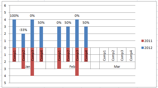
Add % Difference Data Labels to Excel Horizontal Tornado ...
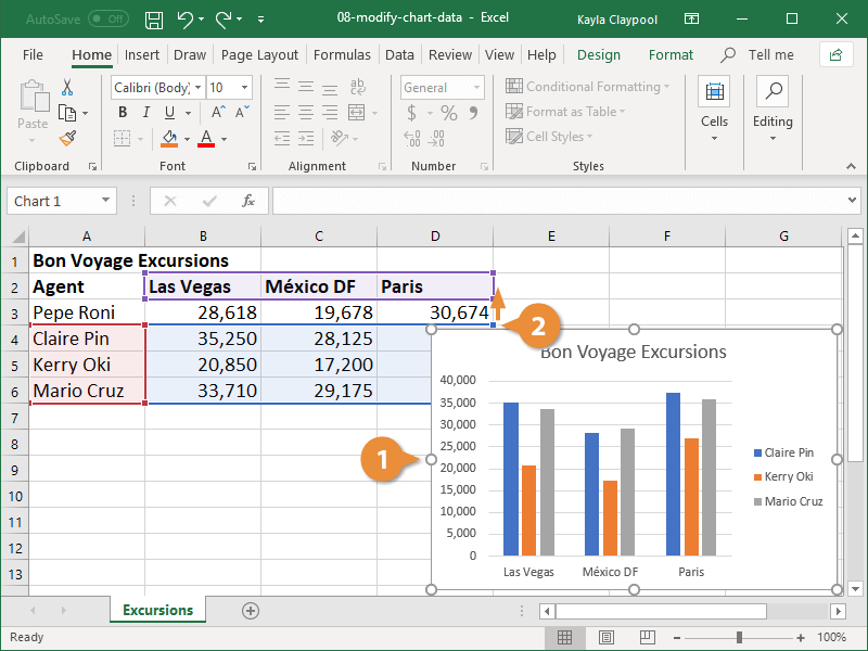
Modify Excel Chart Data Range | CustomGuide

Change the format of data labels in a chart

How To Show Or Hide Data Labels On MS Excel? | My Windows Hub
Move data labels

How to Create a Pie Chart in Excel | Smartsheet
Post a Comment for "45 change order of data labels in excel chart"