42 multiple data labels excel pie chart

Multiple Data Labels on a Pie Chart - MrExcel Message Board This table includes: Column 1 - shipment name. Column 2 - shipment cost. Column 3 - shipment weight. I have created a pie chart from this table, which covers the first two columns. Displayed next to each slice is a label with the shipment name, shipment cost, and percent share of the pie. How to Create a Pie Chart in Excel - Smartsheet Enter data into Excel with the desired numerical values at the end of the list. Create a Pie of Pie chart. Double-click the primary chart to open the Format Data Series window. Click Options and adjust the value for Second plot contains the last to match the number of categories you want in the "other" category.

Adding data labels to a pie chart - Excel General - OzGrid With ActiveChart.SeriesCollection(1) ' HasDataLabels is a valid property .HasDataLabels = True ' XL2000 pie chart .ApplyDataLabels Type:=xlDataLabelsShowPercent _ , AutoText:=True, LegendKey:=False, HasLeaderLines:=True ' XL2003 pie chart ' .ApplyDataLabels AutoText:=True, LegendKey:= _ ' False, HasLeaderLines:=True, ShowSeriesName:=True, 'ShowCategoryName:=True _ ' , ShowValue:=True, ShowPercentage:=True, 'ShowBubbleSize:=False, _ ' Separator:=", " With .DataLabels .Font.Bold = True With ...

Multiple data labels excel pie chart

Edit titles or data labels in a chart - support.microsoft.com The first click selects the data labels for the whole data series, and the second click selects the individual data label. Right-click the data label, and then click Format Data Label or Format Data Labels. Click Label Options if it's not selected, and then select the Reset Label Text check box. Top of Page Solved: Show multiple data lables on a chart - Power BI For example, I'd like to include both the total and the percent on pie chart. Or instead of having a separate legend include the series name along with the % in a pie chart. I know they can be viewed as tool tips, but this is not sufficient for my needs. Many of my charts are copied to presentations and this added data is necessary for the end users. Create two data labels in pie chart? | MrExcel Message Board 30 Aug 2018 — There are 50 pie charts and I don't want to manually adjust each one. Suggestions? Excel Facts.3 answers · 0 votes: Hi, Sorry but maybe I didn’t make that very clear. I intended that you simply put the icon/image ...

Multiple data labels excel pie chart. Pie Chart in Excel | How to Create Pie Chart - EDUCBA Pie Chart in Excel is used for showing the completion or main contribution of different segments out of 100%. It is like each value represents the portion of the Slice from the total complete Pie. For Example, we have 4 values A, B, C and D. Excel Pie Chart Multiple Series - TheRescipes.info Creating Pie of Pie Chart in Excel: Follow the below steps to create a Pie of Pie chart: 1. In Excel, Click on the Insert tab. 2. Click on the drop-down menu of the pie chart from the list of the charts. 3. Move data labels - support.microsoft.com Right-click the selection > Chart Elements > Data Labels arrow, and select the placement option you want. Different options are available for different chart types. For example, you can place data labels outside of the data points in a pie chart but not in a column chart. Quickly create multiple progress pie charts in one graph 1. Click Kutools > Charts > Difference Comparison > Progress Pie Chart to go to the Progress Pie Chart dialog box. 2. In the popped out dialog box, select the data range of the axis labels, actual values and target values under the Axis Labels, Actual Value and Target Value boxes separately. See screenshot:

Create a multi-level category chart in Excel - ExtendOffice 1. Firstly, arrange your data which you will create a multi-level category chart based on as follows. 1.1) In the first column, please type in the main category names; 1.2) In the second column, type in the subcategory names; 1.3) In the third column, type in each data for the subcategories. 2. Creating Pie Chart and Adding/Formatting Data Labels (Excel) Creating Pie Chart and Adding/Formatting Data Labels (Excel) - YouTube. Everything You Need to Know About Pie Chart in Excel Start with selecting your data in Excel. If you include data labels in your selection, Excel will automatically assign them to each column and generate the chart. Go to the INSERT tab in the Ribbon and click on the Pie Chart icon to see the pie chart types. Click on the desired chart to insert. In this example, we're going to be using Pie. How to fix wrapped data labels in a pie chart - Sage Intelligence Right click on the data label and select Format Data Labels. 2. Select Text Options > Text Box > and un-select Wrap text in shape. 3. The data labels resize to fit all the text on one line. 4. Alternatively, by double-clicking a data label, the handles can be used to resize the label to wrap words as desired. This can be done on all data labels ...

How to group (two-level) axis labels in a chart in Excel? Create a Pivot Chart with selecting the source data, and: (1) In Excel 2007 and 2010, clicking the PivotTable > PivotChart in the Tables group on the Insert Tab; (2) In Excel 2013, clicking the Pivot Chart > Pivot Chart in the Charts group on the Insert tab. 2. In the opening dialog box, check the Existing worksheet option, and then select a ... Excel Pie Chart Multiple Labels Formatting data labels and printing pie charts on Excel for Mac … Excel Details: Work around: Select the area of the chart - by selecting the cells behind where the chart is sitting > Print area> Select print area>File > print>then set print perameters (paper … How to display leader lines in pie chart in Excel? - ExtendOffice To display leader lines in pie chart, you just need to check an option then drag the labels out. 1. Click at the chart, and right click to select Format Data Labels from context menu. 2. In the popping Format Data Labels dialog/pane, check Show Leader Lines in the Label Options section. See screenshot: 3. Change the format of data labels in a chart To get there, after adding your data labels, select the data label to format, and then click Chart Elements > Data Labels > More Options. To go to the appropriate area, click one of the four icons ( Fill & Line, Effects, Size & Properties ( Layout & Properties in Outlook or Word), or Label Options) shown here.

Advanced Graphs Using Excel : 3D-histogram in Excel

Multiple data labels (in separate locations on chart) Re: Multiple data labels (in separate locations on chart) The revised example includes screen shots of dialogs for changeing axis and data sources. You can use the Up/Down arrows to move through chart elements in order to select the second pie.

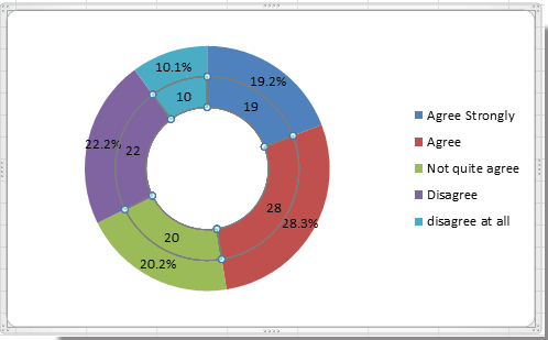
How to create doughnut chart in Excel?

Formatting data labels and printing pie charts on Excel for Mac 2019 ... Here's a work around I found for printing pie charts. Still can't find a solution for formatting the data labels. 1. When printing a pie chart from Excel for mac 2019, MS instructions are to select the chart only, on the worksheet > file > print. Excel is supposed to print the chart only (not the data ) and automatically fit it onto one page.

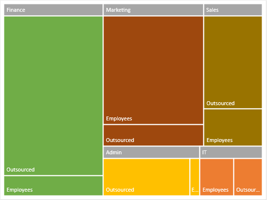
New, better alternative to Pie Charts: Treemap - Efficiency 365

How to add data labels from different column in an Excel chart? This method will guide you to manually add a data label from a cell of different column at a time in an Excel chart. 1. Right click the data series in the chart, and select Add Data Labels > Add Data Labels from the context menu to add data labels. 2. Click any data label to select all data labels, and then click the specified data label to select it only in the chart.

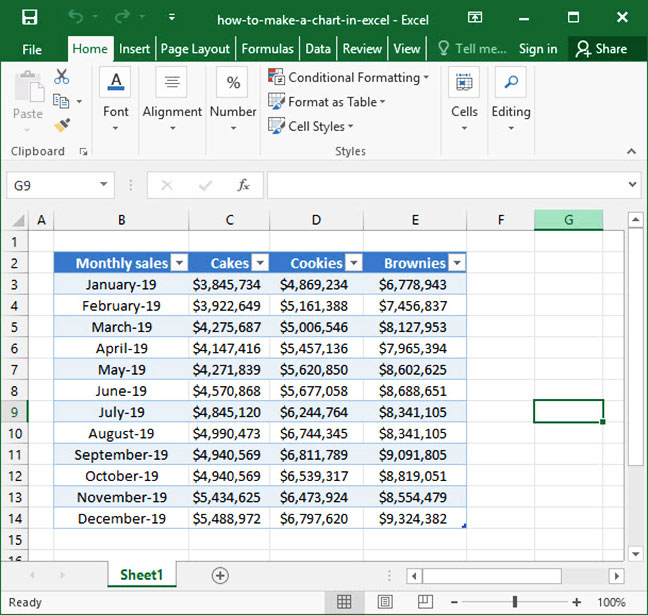
How To Make a Chart In Excel | Deskbright

How to Create and Format a Pie Chart in Excel - Lifewire To create a pie chart, highlight the data in cells A3 to B6 and follow these directions: On the ribbon, go to the Insert tab. Select Insert Pie Chart to display the available pie chart types. Hover over a chart type to read a description of the chart and to preview the pie chart. Choose a chart type.

Share :