44 excel line chart axis labels

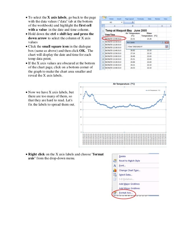
How to add Axis Labels (X & Y) in Excel & Google Sheets Adding Axis Labels. Double Click on your Axis; Select Charts & Axis Titles . 3. Click on the Axis Title you want to Change (Horizontal or Vertical Axis) 4. Type in your Title Name . Axis Labels Provide Clarity. Once you change the title for both axes, the user will now better understand the graph. Change axis labels in a chart - support.microsoft.com Right-click the category labels you want to change, and click Select Data. In the Horizontal (Category) Axis Labels box, click Edit. In the Axis label range box, enter the labels you want to use, separated by commas. For example, type Quarter 1,Quarter 2,Quarter 3,Quarter 4. Change the format of text and numbers in labels

How to Place Labels Directly Through Your Line Graph in Microsoft Excel Select Format Data Labels. In the Format Data Labels editing window, adjust the Label Position. By default the labels appear to the right of each data point. Click on Center so that the labels appear right on top of each point. Umm yeah. So the labels are totally unreadable because they've got a line running through them.

Excel line chart axis labels

Change the display of chart axes - support.microsoft.com charts typically have two axes that are used to measure and categorize data: a vertical axis (also known as value axis or y axis), and a horizontal axis (also known as category axis or x axis). 3-d column, 3-d cone, or 3-d pyramid charts have a third axis, the depth axis (also known as series axis or z axis), so that data can be plotted along the … How to display text labels in the X-axis of scatter chart in ... Display text labels in X-axis of scatter chart. Actually, there is no way that can display text labels in the X-axis of scatter chart in Excel, but we can create a line chart and make it look like a scatter chart. 1. Select the data you use, and click Insert > Insert Line & Area Chart > Line with Markers to select a line chart. See screenshot: How to Create Line Charts in Excel (In Easy Steps) Line charts are used to display trends over time. Use a line chart if you have text labels, dates or a few numeric labels on the horizontal axis. Use a scatter plot (XY chart) to show scientific XY data. To create a line chart, execute the following steps. 1. Select the range A1:D7. 2. On the Insert tab, in the Charts group, click the Line symbol.

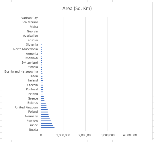
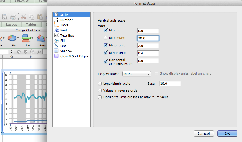
Excel line chart axis labels. Format Chart Axis in Excel - Axis Options Right-click on the Vertical Axis of this chart and select the "Format Axis" option from the shortcut menu. This will open up the format axis pane at the right of your excel interface. Thereafter, Axis options and Text options are the two sub panes of the format axis pane. Formatting Chart Axis in Excel - Axis Options : Sub Panes Present your data in a scatter chart or a line chart This is a good example of when not to use a line chart. A line chart distributes category data evenly along a horizontal (category) axis , and distributes all numerical value data along a vertical (value) axis. The particulate y value of 137 (cell B9) and the daily rainfall x value of 1.9 (cell A9) are displayed as separate data points in the ... Excel tutorial: How to customize axis labels Instead you'll need to open up the Select Data window. Here you'll see the horizontal axis labels listed on the right. Click the edit button to access the label range. It's not obvious, but you can type arbitrary labels separated with commas in this field. So I can just enter A through F. When I click OK, the chart is updated. Dynamically Label Excel Chart Series Lines - My Online Training Hub Step 1: Duplicate the Series. The first trick here is that we have 2 series for each region; one for the line and one for the label, as you can see in the table below: Select columns B:J and insert a line chart (do not include column A). To modify the axis so the Year and Month labels are nested; right-click the chart > Select Data > Edit the ...

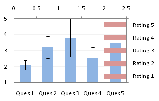
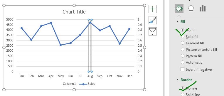
Excel Chart Vertical Axis Text Labels • My Online Training Hub Click on the top horizontal axis and delete it. Hide the left hand vertical axis: right-click the axis (or double click if you have Excel 2010/13) > Format Axis > Axis Options: Set tick marks and axis labels to None. While you're there set the Minimum to 0, the Maximum to 5, and the Major unit to 1. This is to suit the minimum/maximum values ... Chart Axis – Use Text Instead of Numbers – Excel & Google ... Select Data Labels; Click on Arrow and click Left . 4. Double click on each Y Axis line type = in the formula bar and select the cell to reference . 5. Click on the Series and Change the Fill and outline to No Fill . 6. Click on the Original Y Axis Series with numbers and click Delete . Final Graph with Numbers Replaced by Text How to group (two-level) axis labels in a chart in Excel? Select the source data, and then click the Insert Column Chart (or Column) > Column on the Insert tab. Now the new created column chart has a two-level X axis, and in the X axis date labels are grouped by fruits. See below screen shot: Group (two-level) axis labels with Pivot Chart in Excel Add or remove data labels in a chart - support.microsoft.com On the Design tab, in the Chart Layouts group, click Add Chart Element, choose Data Labels, and then click None. Click a data label one time to select all data labels in a data series or two times to select just one data label that you want to delete, and then press DELETE. Right-click a data label, and then click Delete.

Excel tutorial: How to create a multi level axis To straighten out the labels, I need to restructure the data. First, I'll sort by region and then by activity. Next, I'll remove the extra, unneeded entries from the region column. The goal is to create an outline that reflects what you want to see in the axis labels. Now you can see we have a multi level category axis. How To Add Axis Labels In Excel [Step-By-Step Tutorial] First off, you have to click the chart and click the plus (+) icon on the upper-right side. Then, check the tickbox for 'Axis Titles'. If you would only like to add a title/label for one axis (horizontal or vertical), click the right arrow beside 'Axis Titles' and select which axis you would like to add a title/label. Editing the Axis Titles How to rotate axis labels in chart in Excel? - ExtendOffice Rotate axis labels in chart of Excel 2013 If you are using Microsoft Excel 2013, you can rotate the axis labels with following steps: 1. Go to the chart and right click its axis labels you will rotate, and select the Format Axis from the context menu. 2. How to Insert Axis Labels In An Excel Chart | Excelchat How to add vertical axis labels in Excel 2016/2013 We will again click on the chart to turn on the Chart Design tab We will go to Chart Design and select Add Chart Element Figure 6 - Insert axis labels in Excel In the drop-down menu, we will click on Axis Titles, and subsequently, select Primary vertical

32 Excel Chart Axis Label - Labels 2021

Two-Level Axis Labels (Microsoft Excel) Place your row labels into column A, beginning at cell A3. Place your data into the table, beginning at cell B3. With your table completed, you are ready to create the chart. Just select your data table, including all the headings in the first two rows, then create your chart.

Adding Colored Regions to Excel Charts - Duke Libraries Center for Data and Visualization Sciences

How to add axis label to chart in Excel? - ExtendOffice You can insert the horizontal axis label by clicking Primary Horizontal Axis Title under the Axis Title drop down, then click Title Below Axis, and a text box will appear at the bottom of the chart, then you can edit and input your title as following screenshots shown. 4.

Presenting Data with Charts

Custom Axis Labels and Gridlines in an Excel Chart Select the horizontal dummy series and add data labels. In Excel 2007-2010, go to the Chart Tools > Layout tab > Data Labels > More Data Label Options. In Excel 2013, click the "+" icon to the top right of the chart, click the right arrow next to Data Labels, and choose More Options…. Then in either case, choose the Label Contains option ...

Text Labels on a Vertical Column Chart in Excel - Peltier Tech Blog

Label Specific Excel Chart Axis Dates - My Online Training Hub Step 1 - Insert a regular line or scatter chart. I'm going to insert a scatter chart so I can show you another trick most people don't know*. Step 2 - Hide the line for the 'Date Label Position' series: Step 3 - Set the desired minimum and maximum dates (Scatter Charts Only)

microsoft office - Multiple Y-axis labels in Excel 2010 line chart - Super User

How to change chart axis labels' font color and size in Excel? We can easily change all labels' font color and font size in X axis or Y axis in a chart. Just click to select the axis you will change all labels' font color and size in the chart, and then type a font size into the Font Size box, click the Font color button and specify a font color from the drop down list in the Font group on the Home tab.

How to make_a_line_graph_using_excel_2007

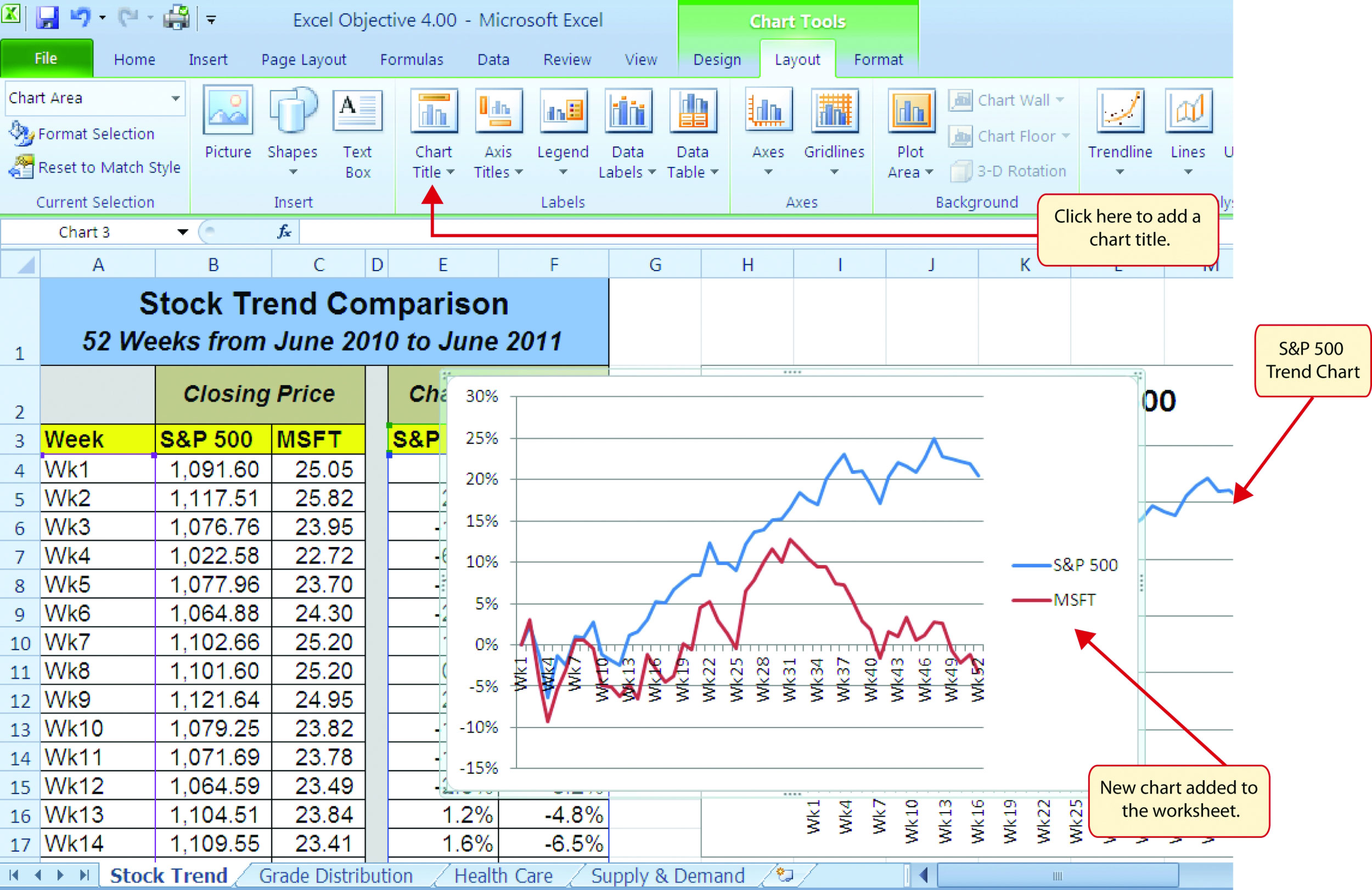
Excel charts: add title, customize chart axis, legend and data labels ... Click anywhere within your Excel chart, then click the Chart Elements button and check the Axis Titles box. If you want to display the title only for one axis, either horizontal or vertical, click the arrow next to Axis Titles and clear one of the boxes: Click the axis title box on the chart, and type the text.

Excel isn't showing some of my Horizontal (Category) Axis Labels - Super User

Excel 2019 will not use text column as X-axis labels Apparently, line chart and bar chart are the only two types of bivariate plots in Excel 2019 that will display categorical axis labels. (I could not get this to work with line-connected scatter plot, following your or myall's steps).

How To Add Axis Labels In Excel [Step-By-Step Tutorial]

How to Make Line Graphs in Excel | Smartsheet Step-by-Step Instructions to Build a Line Graph in Excel. Once you collect the data you want to chart, the first step is to enter it into Excel. The first column will be the time segments (hour, day, month, etc.), and the second will be the data collected (muffins sold, etc.). Highlight both columns of data and click Charts > Line > and make ...

How to Insert Axis Labels In An Excel Chart | Excelchat

Excel tutorial: How to reverse a chart axis In this video, we'll look at how to reverse the order of a chart axis. Here we have data for the top 10 islands in the Caribbean by population. Let me insert a standard column chart and let's look at how Excel plots the data. When Excel plots data in a column chart, the labels run from left to right to left.

Excel charts: add title, customize chart axis, legend and data labels

Change axis labels in a chart in Office - support.microsoft.com In charts, axis labels are shown below the horizontal (also known as category) axis, next to the vertical (also known as value) axis, and, in a 3-D chart, next to the depth axis. The chart uses text from your source data for axis labels. To change the label, you can change the text in the source data.

33 How To Label Axis In Excel - Labels Database 2020

How to wrap X axis labels in a chart in Excel? - ExtendOffice And you can do as follows: 1. Double click a label cell, and put the cursor at the place where you will break the label. 2. Add a hard return or carriages with pressing the Alt + Enter keys simultaneously. 3. Add hard returns to other label cells which you want the labels wrapped in the chart axis.

Line Graph in Microsoft Excel

How to Label Axes in Excel: 6 Steps (with Pictures) - wikiHow 2 Select the graph. Click your graph to select it. 3 Click +. It's to the right of the top-right corner of the graph. This will open a drop-down menu. 4 Click the Axis Titles checkbox. It's near the top of the drop-down menu. Doing so checks the Axis Titles box and places text boxes next to the vertical axis and below the horizontal axis.

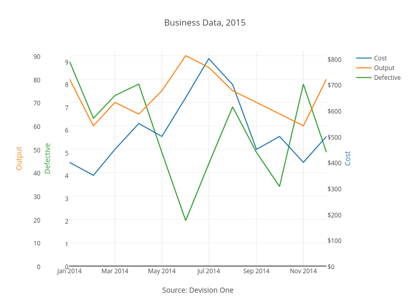
Three Y Axes Graph with Chart Studio and Excel

How to Create Line Charts in Excel (In Easy Steps) Line charts are used to display trends over time. Use a line chart if you have text labels, dates or a few numeric labels on the horizontal axis. Use a scatter plot (XY chart) to show scientific XY data. To create a line chart, execute the following steps. 1. Select the range A1:D7. 2. On the Insert tab, in the Charts group, click the Line symbol.

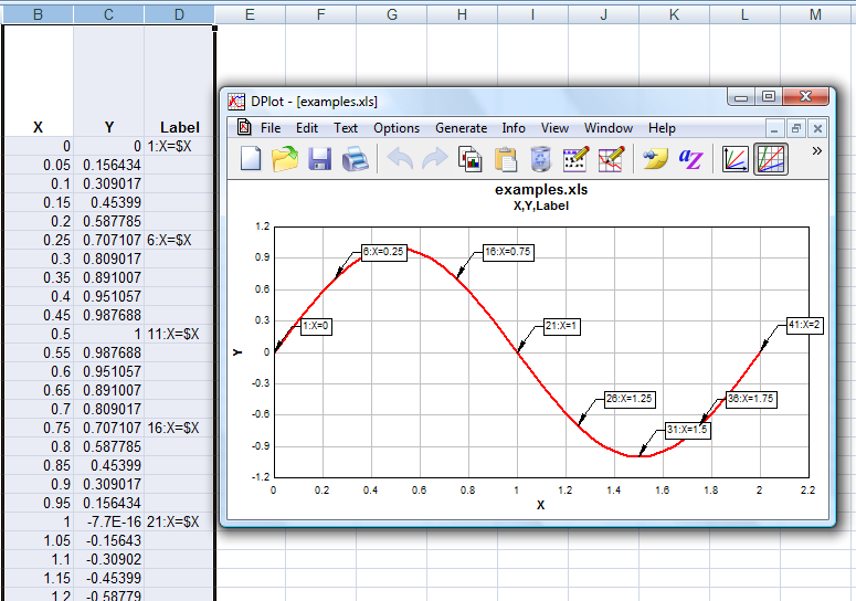
DPlot Windows software for Excel users to create presentation quality graphs

How to display text labels in the X-axis of scatter chart in ... Display text labels in X-axis of scatter chart. Actually, there is no way that can display text labels in the X-axis of scatter chart in Excel, but we can create a line chart and make it look like a scatter chart. 1. Select the data you use, and click Insert > Insert Line & Area Chart > Line with Markers to select a line chart. See screenshot: