40 excel chart labels from cells

How to Show Percentages in Stacked Column Chart in Excel ... By default, the data labels are shown in the form of chart data Value (Image 1). But very often user needs to plot charts with actual data and show percentages/custom values on the chart instead of default data. For that we have an option "Value From Cells" in chart "Format Data Label" (Image 2) to select a custom range. Image 1 Image 2 Gnatt chart - list cells from 'tasks' columns based on ... Gnatt chart - list cells from 'tasks' columns based on date. See the example sheet attached. I have a Gantt chart with a list of tasks on the right and dates along the top. On a new sheet, I would like to be able to select a date range with the result being a list of tasks that are active within that date range.

Chart.ApplyDataLabels method (Excel) | Microsoft Docs For the Chart and Series objects, True if the series has leader lines. Pass a Boolean value to enable or disable the series name for the data label. Pass a Boolean value to enable or disable the category name for the data label. Pass a Boolean value to enable or disable the value for the data label.

Excel chart labels from cells

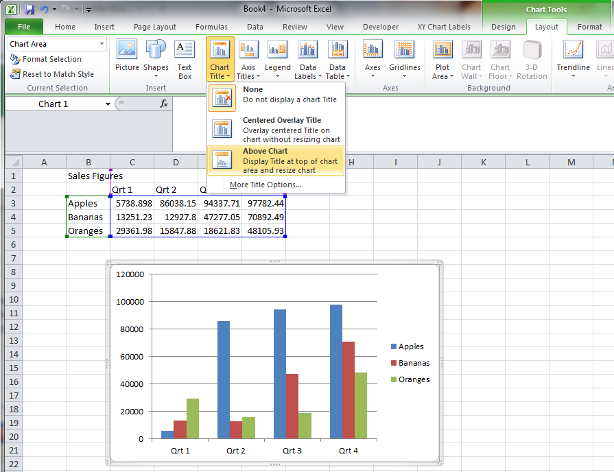
Custom Chart Data Labels In Excel With Formulas Follow the steps below to create the custom data labels. Select the chart label you want to change. In the formula-bar hit = (equals), select the cell reference containing your chart label's data. In this case, the first label is in cell E2. Finally, repeat for all your chart laebls. How to Create Multi-Category Charts in Excel ... Step 1: Insert the data into the cells in Excel. Now select all the data by dragging and then go to "Insert" and select "Insert Column or Bar Chart". A pop-down menu having 2-D and 3-D bars will occur and select "vertical bar" from it. Select the cell -> Insert -> Chart Groups -> 2-D Column Bar Chart Insertion Multi-Category Chart How To Add Axis Labels In Excel [Step-By-Step Tutorial] First off, you have to click the chart and click the plus (+) icon on the upper-right side. Then, check the tickbox for 'Axis Titles'. If you would only like to add a title/label for one axis (horizontal or vertical), click the right arrow beside 'Axis Titles' and select which axis you would like to add a title/label. Editing the Axis Titles

Excel chart labels from cells. How to Add Labels to Scatterplot Points in Excel - Statology Next, click anywhere on the chart until a green plus (+) sign appears in the top right corner. Then click Data Labels, then click More Options… In the Format Data Labels window that appears on the right of the screen, uncheck the box next to Y Value and check the box next to Value From Cells. How to Make and Print Labels from Excel with Mail Merge How to mail merge labels from Excel Open the "Mailings" tab of the Word ribbon and select "Start Mail Merge > Labels…". The mail merge feature will allow you to easily create labels and import data... How to Print Labels from Excel - Lifewire To label legends in Excel, select a blank area of the chart, select the Plus ( +) in the upper-right, and check the Legend checkbox. Then, select the cell containing the legend and enter a new name. How do I label a series in Excel? To label a series in Excel, right-click the chart with the data series and choose Select Data. Two-Level Axis Labels (Microsoft Excel) Excel automatically recognizes that you have two rows being used for the X-axis labels, and formats the chart correctly. Since the X-axis labels appear beneath the chart data, the order of the label rows is reversed—exactly as mentioned at the first of this tip. (See Figure 1.) Figure 1. Two-level axis labels are created automatically by Excel.

› documents › excelHow to wrap X axis labels in a chart in Excel? Some users may want to wrap the labels in the chart axis only, but not wrap the label cells in the source data. Actually, we can replace original labels cells with formulas in Excel. For example, you want to wrap the label of "OrangeBBBB" in the axis, just find out the label cell in the source data, and then replace the original label with the ... Improve your X Y Scatter Chart with custom data labels Press with right mouse button on on a chart dot and press with left mouse button on on "Add Data Labels" Press with right mouse button on on any dot again and press with left mouse button on "Format Data Labels" A new window appears to the right, deselect X and Y Value. Enable "Value from cells" Select cell range D3:D11 › Utilities › ChartLabelerThe XY Chart Labeler Add-in - AppsPro Jul 01, 2007 · The XY Chart Labeler. A very commonly requested Excel feature is the ability to add labels to XY chart data points. The XY Chart Labeler adds this feature to Excel. The XY Chart Labeler provides the following options: Add XY Chart Labels - Adds labels to the points on your XY Chart data series based on any range of cells in the workbook. Creating a pie chart in excel with single values rather ... I am trying to create a pie chart in excel, I want each column in the pie chart to be pulled from a single cell in my excel work book rather than from a table. When I try creating a pie chart it only lets me create it via a series, is there a way that I can make a pie chart without needing to create a table for it to pull from?

Slope Chart with Data Labels - Peltier Tech In Format all data labels at once on the Mr Excel forum, a user was frustrated with having to format data labels on his slope chart one point at a time, which is a very tedious and frustrating experience.One solution to such tedious tasks is VBA, and I wrote a procedure that would apply and format all data labels at once. The procedure ran instantly, compared to the many minutes it would take ... Format Chart Axis in Excel - Axis Options (Format Axis ... Right-click on the Vertical Axis of this chart and select the "Format Axis" option from the shortcut menu. This will open up the format axis pane at the right of your excel interface. Thereafter, Axis options and Text options are the two sub panes of the format axis pane. Formatting Chart Axis in Excel - Axis Options : Sub Panes Series.DataLabels method (Excel) | Microsoft Docs Return value. Object. Remarks. If the series has the Show Value option turned on for the data labels, the returned collection can contain up to one label for each point. Data labels can be turned on or off for individual points in the series. If the series is on an area chart and has the Show Label option turned on for the data labels, the returned collection contains only a single label ... How to ☝️Change the Position and Size of Excel Charts in ... Here's the breakdown of the code we added to help you adjust..Height = Range("A1:A20").Height - This line of code sets the height of your graph using worksheet cells as a measuring tool.In this example, the chart height equals the distance from cell D5 to cell D25..Width = Range("A1:E1").Width - This determines the width of your chart.. As for the pie chart we used as a running ...

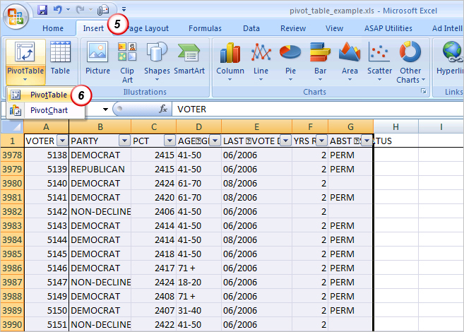
In Search of the Elusive Pivot Table | Dynamic Edge, Inc. | Beyond Tech Support Dynamic Edge ...

50 Excel Shortcuts That You Should Know in 2022 Cell Formatting Shortcut Keys. A cell in Excel holds all the data that you are working on. Several different shortcuts can be applied to a cell, such as editing a cell, aligning cell contents, adding a border to a cell, adding an outline to all the selected cells, and many more. Here is a sneak peek into these Excel shortcuts.

Timeline Chart in Excel - Goodly

Pie Chart in Excel - Inserting, Formatting, Filtering ... Right click on the Data Labels on the chart. Click on Format Data Labels option. Consequently, this will open up the Format Data Labels pane on the right of the excel worksheet. Mark the Category Name, Percentage and Legend Key. Also mark the labels position at Outside End. This is how the chark looks. Formatting the Chart Background, Chart Styles

Add Custom Labels to x-y Scatter plot in Excel - DataScience Made Simple

chandoo.org › wp › budget-vs-actual-chart-free-templateFree Budget vs. Actual chart Excel Template - Download May 16, 2018 · Step 12: Plug our smart labels in to the chart. Now that we have gorgeous labels, let’s replace the old ones with these. Select first line (budget)’s labels and press CTRL+1 to go to format options. Click on “Value from cells” option and point to Var 1 column. Repeat the process for second line (actual) labels too. We get this.

Excel Is Fun

Excel: How To Convert Data Into A Chart/Graph - Digital ... 7: To add axis titles, data labels, legend, trendline, and more, click the graph you just created. A new tab titled "Chart design" should appear. In the upper menu of that tab, you should see a section called "add chart element." 8: In "add chart element," you can customize your graph to your liking . STEP 9: Don't forget to save your work!

Fill Blank Cells With Value Above or Below the Cell or Zero | Excel Solutions - Basic and Advanced

How To Create a Burndown Chart in Excel (With Benefits ... Open a new spreadsheet in Excel and create labels for your data. In a simple layout, use the first row for your labels. Combine cells A1 and B1 and label the new cell "timeline" to create a double column under A and B. Use cell A2 for the "date" and cell B2 for the "day" to track the actual working days you complete the sprint tasks.

How to Use Cell Values for Excel Chart Labels

Data label in the graph not showing percentage option ... Re: Data label in the graph not showing percentage option. only value coming. @Dipil. You need helper columns but you don't need another chart. Add columns with percentage and use "Values from cells" option to add it as data labels. labels percent.xlsx. Preview file.

How to Change Horizontal Axis Labels in Excel 2010 - Solve Your Tech

I do not want to show data in chart that is "0" (zero ... Excel charts have options that control how they will respond to hidden and empty cells. Cells that are left blank are treated as empty cells. To access these options, select the chart and click: Chart Tools > Design > Select Data > Hidden and Empty Cells You can use these settings to control whether empty cells are shown as gaps or zeros on charts.

Excel Data Labels - Value from Cells

How to☝️ Make a Professional Gantt Chart in Excel [2 FREE ... How to Make a Gantt Chart in Excel Daniel Smith August 12, 2021 This Article Contains: Step 1. Add the Project Data Step 2. Prepare the Gantt Chart Data Step 3. Create a Stacked Column Chart Step 4. Add New Data Series Step 5. Modify the Vertical Axis (Add the Tasks) Step 6. Reverse the Category Order Step 7. Create a Gantt Chart Step 8.

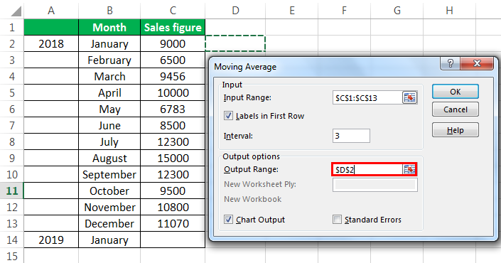
Calculate Moving Average in Excel (Simple, Exponential and Weighted)

Prevent Overlapping Data Labels in Excel Charts - Peltier Tech Apply Data Labels to Charts on Active Sheet, and Correct Overlaps Can be called using Alt+F8 ApplySlopeChartDataLabelsToChart (cht As Chart) Apply Data Labels to Chart cht Called by other code, e.g., ApplySlopeChartDataLabelsToActiveChart FixTheseLabels (cht As Chart, iPoint As Long, LabelPosition As XlDataLabelPosition)

Variance Analysis in Excel - Making better Budget Vs Actual charts - PakAccountants.com

How to Create and Customize a Waterfall Chart in Microsoft ... Select the chart and use the buttons on the right (Excel on Windows) to adjust Chart Elements like labels and the legend, or Chart Styles to pick a theme or color scheme. Select the chart and go to the Chart Design tab. Then, use the tools in the ribbon to select a different layout, change the colors, pick a new style, or adjust your data ...

Positive Negative Bar Chart - Beat Excel!

How to Create a Bar Chart in Excel with Multiple Bars ... To fine tune the bar chart in excel, you can add a title to the graph. You can also add data labels. To add data labels, go to the Chart Design ribbon, and from the Add Chart Element, options select Add Data Labels. Adding data labels will add an extra flair to your graph. You can compare the score more easily and come to a conclusion faster.

MS Excel 2013: Create a superscript value in a cell

› charts › variance-clusteredActual vs Budget or Target Chart in Excel - Variance on ... Aug 19, 2013 · Next you will right click on any of the data labels in the Variance series on the chart (the labels that are currently displaying the variance as a number), and select “Format Data Labels” from the menu. On the right side of the screen you should see the Label Options menu and the first option is “Value From Cells”.

34 Cell Label Excel - Labels Design Ideas 2020

How to Insert a Legend in Excel Based on Cell Colors Select the whole range and click on "Filter" on the Data ribbon. Then, click on the small filter icon in the heading of a column and scroll down to "Filter by Color". Now, you can see all different colors used in the column. Method 2: Use a VBA macro to insert a table of all background colors Our next method to insert a legend involves a VBA macro.

Automatically hide labels in line chart if cell is blank - Excel - Stack Overflow

How to add text or specific character to Excel cells ... How to add special character to cell in Excel. To insert a special character in an Excel cell, you need to know its code in the ASCII system. Once the code is established, supply it to the CHAR function to return a corresponding character. The CHAR function accepts any number from 1 to 255.

Using Labels to Simplify Your Excel 2003 Formulas

How To Add Axis Labels In Excel [Step-By-Step Tutorial] First off, you have to click the chart and click the plus (+) icon on the upper-right side. Then, check the tickbox for 'Axis Titles'. If you would only like to add a title/label for one axis (horizontal or vertical), click the right arrow beside 'Axis Titles' and select which axis you would like to add a title/label. Editing the Axis Titles

How to count cells that contain values in Excel | Basic Excel Tutorial

How to Create Multi-Category Charts in Excel ... Step 1: Insert the data into the cells in Excel. Now select all the data by dragging and then go to "Insert" and select "Insert Column or Bar Chart". A pop-down menu having 2-D and 3-D bars will occur and select "vertical bar" from it. Select the cell -> Insert -> Chart Groups -> 2-D Column Bar Chart Insertion Multi-Category Chart

Share :